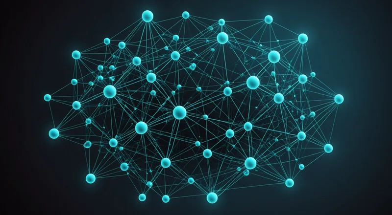
Graph neural networks have become the dominant architecture for crystal property prediction in the past several years, largely displacing earlier descriptor-based approaches (fingerprints, Coulomb matrices, structure-based feature vectors) for most property prediction tasks. The reason is architectural fit: a crystal is naturally represented as a graph, and graph neural networks are explicitly built to learn from graph-structured data. But "naturally represented as a graph" is doing a lot of work in that sentence, and the details of how you construct the graph and how the network processes it determine most of what matters about model quality.
This is a working overview aimed at materials R&D teams who are using or evaluating GNN-based property models and need to understand enough about the architecture to make informed decisions about which models to trust for which tasks. It is not a review of the research literature; it is a description of what the architecture does and where it tends to go wrong.
Representing a Crystal as a Graph
The most important property of a crystal structure for property prediction is the local chemical environment around each atom: what species are nearby, how far away they are, and what angles the bonds form. A graph representation encodes this by treating each atom as a node and each interatomic interaction as an edge.
Node features
Node features encode information about each atom type. The simplest version is a one-hot encoding of element identity. More informative encodings include atomic number, period, group, electronegativity, ionic radius, oxidation state (if known), and whether the atom sits on a symmetry-distinct site. The choice of initial node features affects model expressiveness, particularly for distinguishing chemically similar elements that differ in more subtle properties.
Edge features and cutoff radius
Each edge represents an interatomic distance within a specified cutoff radius. The cutoff radius determines which atom pairs become edges and is a critical hyperparameter. Too small a cutoff and you miss medium-range interactions that are important for structural stability (particularly in ionic compounds where next-nearest-neighbor interactions are significant). Too large a cutoff and the graph becomes dense, the message-passing updates are dominated by distant atoms that contribute little signal, and training is slower.
In practice, cutoff radii between 4 and 8 angstroms cover most chemically relevant interactions for inorganic compounds. Models trained on oxide cathodes typically use 5 to 6 angstroms. Models intended to cover more ionic crystal classes often use 6 to 8 angstroms. Beyond the cutoff radius, edge features typically encode the interatomic distance (as a Gaussian basis expansion or Bessel function embedding) and, in angle-aware architectures, the bond angles at shared atoms.
Periodic boundary conditions
Crystals are periodic. A graph representation must account for the fact that an atom near the edge of the unit cell has neighbors in adjacent unit cells. This is handled by including image atoms: when constructing edges, you include bonds to periodic images of atoms in the neighboring unit cells, up to the cutoff radius. The resulting graph is finite even though the physical structure is infinite. Most GNN implementations for crystalline materials handle this correctly, but it is worth verifying for any model you use that the periodic boundary handling is implemented for your system's crystal symmetry.
Message Passing: How the Network Learns from the Graph
The defining operation in a graph neural network is message passing. In each layer, every node aggregates information from its neighbors, updates its own representation based on that aggregation, and passes the updated representation forward to the next layer. Over multiple layers, a node's representation incorporates information from increasingly distant neighbors: after one layer, each node knows about its immediate neighbors; after two layers, it knows about its neighbors' neighbors; and so on.
For property prediction, the key design choices are:
- Message function: How is the information from a neighbor combined with the edge features before being aggregated? The message function determines how much the bond geometry (distance, angles) influences the update, versus just the neighbor's current representation.
- Aggregation function: How are messages from multiple neighbors combined into a single update signal? Sum aggregation is most common. Mean aggregation is less sensitive to coordination number differences but loses information about the total number of neighbors, which matters for properties that depend on coordination.
- Update function: How is the aggregated message combined with the node's current representation to produce the updated representation? Typically a learned transformation with a nonlinear activation.
The number of message-passing layers determines the receptive field: how many bonds away from a given atom the model can incorporate information from in a single forward pass. Three to five layers is typical for most crystal property models. More layers increase expressivity but also increase the risk of oversmoothing, where all node representations converge to similar values regardless of local structure, because they incorporate too much long-range context.
Equivariance and Its Practical Importance
A well-designed property model should predict the same energy for a crystal rotated in space as for the original orientation. This is not automatic: naive graph representations that use Cartesian coordinates as edge features will assign different values to the same physical structure at different orientations, which is wrong.
Earlier models addressed this by using only scalar features (interatomic distances) that are rotation-invariant by construction. The limitation is that scalar distances alone cannot distinguish all crystallographically distinct local environments: two different coordination geometries can have the same set of bond distances.
Equivariant architectures (such as NequIP, MACE, and related models) extend message passing to include directional information in a way that correctly transforms when the structure is rotated. The message features include tensorial quantities (vectors, rank-2 tensors) that rotate with the structure, and the model learns to combine these in ways that produce rotation-equivariant outputs. For energy and force prediction, equivariant architectures typically achieve significantly lower prediction error than invariant architectures at the same training set size, which translates directly to better screening accuracy for a given DFT budget.
For inorganic crystal screening where you want to predict atomic forces (not just formation energy), equivariance is important: forces are vectors and must rotate correctly with the structure. If you are using a model that predicts forces for molecular dynamics or geometry optimization, equivariance is not optional.
Where GNNs for Crystals Break Down
Training distribution boundary
The most common failure mode is the same as for any machine learning model: prediction quality degrades outside the training distribution. For crystal property models, this typically manifests as overconfident predictions on composition classes that were rare or absent in the training set. A model trained primarily on ternary oxides will produce plausible-looking but potentially inaccurate predictions on quaternary phosphates unless the training set includes adequate coverage of that chemical space.
This is not a flaw specific to GNNs; it is true of any interpolative model. But the way GNNs fail can be subtle: the model will not obviously "look wrong" on out-of-distribution structures. It will produce a number that is within a reasonable range for the property type. The only reliable way to detect this failure mode is to maintain a held-out validation set that matches your target chemistry and to check model performance on it explicitly before trusting predictions from a screen.
Long-range interactions
Message passing with a finite cutoff radius cannot capture long-range electrostatic or dispersion interactions that extend well beyond typical cutoffs. For most covalently bonded or ionically dominated inorganic materials, the short-to-medium range interactions captured within 5 to 8 angstroms dominate the energy. But for layered materials where interlayer interactions are relevant (graphite intercalation compounds, MXenes, layered sulfides), or for highly polar materials where Madelung energies have long tails, the finite cutoff can introduce systematic errors.
Amorphous and disordered structures
GNNs trained on periodic crystalline structures do not automatically generalize to amorphous phases or structures with significant disorder. An amorphous phase lacks the periodic boundary conditions that the standard graph construction assumes. Disordered structures require either explicit modeling of the disorder or virtual crystal approximations that may not accurately capture the local environment distribution. If your screening target includes amorphous candidates, the standard crystalline GNN architecture is not the right tool without modification.
What This Means for Screening Workflows
The practical implication for materials teams using GNN-based screening is that model architecture matters less than training data coverage and calibration for your specific target chemistry. An older invariant model with good training data coverage for your composition space will outperform a state-of-the-art equivariant foundation model with sparse training coverage for that space.
When evaluating a GNN model for your screening application, the questions worth asking are: what was the training set composition space, what is the per-element training coverage, what is the held-out MAE on a test set drawn from your target chemistry, and does the model provide an uncertainty estimate that you can use as a quality gate. The uncertainty question is especially important: a model that quantifies its own prediction confidence lets you build a screening pipeline that handles high-confidence and low-confidence predictions differently, which is better than treating all predictions as equally reliable.
We use equivariant message-passing architectures in the AstraIQ screening engine because of their force prediction accuracy, and we maintain composition-class-specific validation sets for the material families we serve. The details of how we calibrate uncertainty estimates and use them in the synthesis dispatch queue are described in more detail on the science page. The broader point is that the architecture is a means, not an end: what you build on top of it, in terms of training data curation, validation, and uncertainty handling, is what determines whether the screen is trustworthy.